Compute Shader
Introduction
In this bonus chapter we'll take a look at compute shaders. Up until now all previous chapters dealt with the traditional graphics part of the Vulkan pipeline. But unlike older APIs like OpenGL, compute shader support in Vulkan is mandatory. This means that you can use compute shaders on every Vulkan implementation available, no matter if it's a high-end desktop GPU or a low-powered embedded device.
This opens up the world of general purpose computing on graphics processor units (GPGPU), no matter where your application is running. GPGPU means that you can do general computations on your GPU, something that has traditionally been a domain of CPUs. But with GPUs having become more and more powerful and more flexible, many workloads that would require the general purpose capabilities of a CPU can now be done on the GPU in realtime.
A few examples of where the compute capabilities of a GPU can be used are image manipulation, visibility testing, post processing, advanced lighting calculations, animations, physics (e.g. for a particle system) and much more. And it's even possible to use compute for non-visual computational only work that does not require any graphics output, e.g. number crunching or AI related things. This is called "headless compute".
Advantages
Doing computationally expensive calculations on the GPU has several advantages. The most obvious one is offloading work from the CPU. Another one is not requiring moving data between the CPU's main memory and the GPU's memory. All of the data can stay on the GPU without having to wait for slow transfers from main memory.
Aside from these, GPUs are heavily parallelized with some of them having tens of thousands of small compute units. This often makes them a better fit for highly parallel workflows than a CPU with a few large compute units.
The Vulkan pipeline
It's important to know that compute is completely separated from the graphics part of the pipeline. This is visible in the following block diagram of the Vulkan pipeline from the official specification:
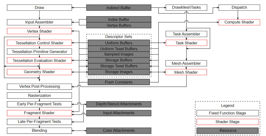
In this diagram we can see the traditional graphics part of the pipeline on the left, and several stages on the right that are not part of this graphics pipeline, including the compute shader (stage). With the compute shader stage being detached from the graphics pipeline we'll be able to use it anywhere we see fit. This is very different from e.g. the fragment shader which is always applied to the transformed output of the vertex shader.
The center of the diagram also shows that e.g. descriptor sets are also used by compute, so everything we learned about descriptors layouts, descriptor sets and descriptors also applies here.
An example
An easy to understand example that we will implement in this chapter is a GPU based particle system. Such systems are used in many games and often consist of thousands of particles that need to be updated at interactive frame rates. Rendering such a system requires 2 main components: vertices, passed as vertex buffers, and a way to update them based on some equation.
The "classical" CPU based particle system would store particle data in the system's main memory and then use the CPU to update them. After the update, the vertices need to be transferred to the GPU's memory again so it can display the updated particles in the next frame. The most straight-forward way would be recreating the vertex buffer with the new data for each frame. This is obviously very costly. Depending on your implementation, there are other options like mapping GPU memory so it can be written by the CPU (called "resizable BAR" on desktop systems, or unified memory on integrated GPUs) or just using a host local buffer (which would be the slowest method due to PCI-E bandwidth). But no matter what buffer update method you choose, you always require a "round-trip" to the CPU to update the particles.
With a GPU based particle system, this round-trip is no longer required. Vertices are only uploaded to the GPU at the start and all updates are done in the GPU's memory using compute shaders. One of the main reasons why this is faster is the much higher bandwidth between the GPU and it's local memory. In a CPU based scenario, you'd be limited by main memory and PCI-express bandwidth, which is often just a fraction of the GPU's memory bandwidth.
When doing this on a GPU with a dedicated compute queue, you can update particles in parallel to the rendering part of the graphics pipeline. This is called "async compute", and is an advanced topic not covered in this tutorial.
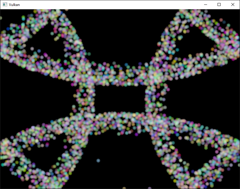
Here is a screenshot from this chapter's code. The particles shown here are updated by a compute shader directly on the GPU, without any CPU interaction:
Data manipulation
In this tutorial we already learned about different buffer types like vertex and index buffers for passing primitives and uniform buffers for passing data to a shader. And we also used images to do texture mapping. But up until now, we always wrote data using the CPU and only did reads on the GPU.
An important concept introduced with compute shaders is the ability to arbitrarily read from and write to buffers. For this, Vulkan offers two dedicated storage types.
Shader storage buffer objects (SSBO)
A shader storage buffer (SSBO) allows shaders to read from and write to a buffer. Using these is similar to using uniform buffer objects. The biggest differences are that you can alias other buffer types to SSBOs and that they can be arbitrarily large.
Going back to the GPU based particle system, you might now wonder how to deal with vertices being updated (written) by the compute shader and read (drawn) by the vertex shader, as both usages would seemingly require different buffer types.
But that's not the case. In Vulkan you can specify multiple usages for buffers and images. So for the particle vertex buffer to be used as a vertex buffer (in the graphics pass) and as a storage buffer (in the compute pass), you simply create the buffer with those two usage flags:
VkBufferCreateInfo bufferInfo{};
...
bufferInfo.usage = VK_BUFFER_USAGE_VERTEX_BUFFER_BIT | VK_BUFFER_USAGE_STORAGE_BUFFER_BIT | VK_BUFFER_USAGE_TRANSFER_DST_BIT;
...

if (vkCreateBuffer(device, &bufferInfo, nullptr, &shaderStorageBuffers[i]) != VK_SUCCESS) {
    throw std::runtime_error("failed to create vertex buffer!");
}
The two flags VK_BUFFER_USAGE_VERTEX_BUFFER_BIT and VK_BUFFER_USAGE_STORAGE_BUFFER_BIT set with bufferInfo.usage tell the implementation that we want to use this buffer for two different scenarios: as a vertex buffer in the vertex shader and as a store buffer. Note that we also added the VK_BUFFER_USAGE_TRANSFER_DST_BIT flag in here so we can transfer data from the host to the GPU. This is crucial as we want the shader storage buffer to stay in GPU memory only (VK_MEMORY_PROPERTY_DEVICE_LOCAL_BIT) we need to to transfer data from the host to this buffer.
Here is the same code using using the createBuffer helper function:
createBuffer(bufferSize, VK_BUFFER_USAGE_STORAGE_BUFFER_BIT | VK_BUFFER_USAGE_VERTEX_BUFFER_BIT | VK_BUFFER_USAGE_TRANSFER_DST_BIT, VK_MEMORY_PROPERTY_DEVICE_LOCAL_BIT, shaderStorageBuffers[i], shaderStorageBuffersMemory[i]);
The GLSL shader declaration for accessing such a buffer looks like this:
struct Particle {
  vec2 position;
  vec2 velocity;
  vec4 color;
};

layout(std140, binding = 1) readonly buffer ParticleSSBOIn {
   Particle particlesIn[ ];
};

layout(std140, binding = 2) buffer ParticleSSBOOut {
   Particle particlesOut[ ];
};
In this example we have a typed SSBO with each particle having a position and velocity value (see the Particle struct). The SSBO then contains an unbound number of particles as marked by the []. Not having to specify the number of elements in an SSBO is one of the advantages over e.g. uniform buffers. std140 is a memory layout qualifier that determines how the member elements of the shader storage buffer are aligned in memory. This gives us certain guarantees, required to map the buffers between the host and the GPU.
Writing to such a storage buffer object in the compute shader is straight-forward and similar to how you'd write to the buffer on the C++ side:
particlesOut[index].position = particlesIn[index].position + particlesIn[index].velocity.xy * ubo.deltaTime;
Storage images
Note that we won't be doing image manipulation in this chapter. This paragraph is here to make readers aware that compute shaders can also be used for image manipulation.
A storage image allows you read from and write to an image. Typical use cases are applying image effects to textures, doing post processing (which in turn is very similar) or generating mip-maps.
This is similar for images:
VkImageCreateInfo imageInfo {};
...
imageInfo.usage = VK_IMAGE_USAGE_SAMPLED_BIT | VK_IMAGE_USAGE_STORAGE_BIT;
...

if (vkCreateImage(device, &imageInfo, nullptr, &textureImage) != VK_SUCCESS) {
    throw std::runtime_error("failed to create image!");
}
The two flags VK_IMAGE_USAGE_SAMPLED_BIT and VK_IMAGE_USAGE_STORAGE_BIT set with imageInfo.usage tell the implementation that we want to use this image for two different scenarios: as an image sampled in the fragment shader and as a storage image in the computer shader;
The GLSL shader declaration for storage image looks similar to sampled images used e.g. in the fragment shader:
layout (binding = 0, rgba8) uniform readonly image2D inputImage;
layout (binding = 1, rgba8) uniform writeonly image2D outputImage;
A few differences here are additional attributes like rgba8 for the format of the image, the readonly and writeonly qualifiers, telling the implementation that we will only read from the input image and write to the output image. And last but not least we need to use the image2D type to declare a storage image.
Reading from and writing to storage images in the compute shader is then done using imageLoad and imageStore:
vec3 pixel = imageLoad(inputImage, ivec2(gl_GlobalInvocationID.xy)).rgb;
imageStore(outputImage, ivec2(gl_GlobalInvocationID.xy), pixel);
Compute queue families
In the physical device and queue families chapter we already learned about queue families and how to select a graphics queue family. Compute uses the queue family properties flag bit VK_QUEUE_COMPUTE_BIT. So if we want to do compute work, we need to get a queue from a queue family that supports compute.
Note that Vulkan requires an implementation which supports graphics operations to have at least one queue family that supports both graphics and compute operations, but it's also possible that implementations offer a dedicated compute queue. This dedicated compute queue (that does not have the graphics bit) hints at an asynchronous compute queue. To keep this tutorial beginner friendly though, we'll use a queue that can do both graphics and compute operations. This will also save us from dealing with several advanced synchronization mechanisms.
For our compute sample we need to change the device creation code a bit:
uint32_t queueFamilyCount = 0;
vkGetPhysicalDeviceQueueFamilyProperties(device, &queueFamilyCount, nullptr);

std::vector<VkQueueFamilyProperties> queueFamilies(queueFamilyCount);
vkGetPhysicalDeviceQueueFamilyProperties(device, &queueFamilyCount, queueFamilies.data());

int i = 0;
for (const auto& queueFamily : queueFamilies) {
    if ((queueFamily.queueFlags & VK_QUEUE_GRAPHICS_BIT) && (queueFamily.queueFlags & VK_QUEUE_COMPUTE_BIT)) {
        indices.graphicsAndComputeFamily = i;
    }

    i++;
}
The changed queue family index selection code will now try to find a queue family that supports both graphics and compute.
We can then get a compute queue from this queue family in createLogicalDevice:
vkGetDeviceQueue(device, indices.graphicsAndComputeFamily.value(), 0, &computeQueue);
The compute shader stage
In the graphics samples we have used different pipeline stages to load shaders and access descriptors. Compute shaders are accessed in a similar way by using the VK_SHADER_STAGE_COMPUTE_BIT pipeline. So loading a compute shader is just the same as loading a vertex shader, but with a different shader stage. We'll talk about this in detail in the next paragraphs. Compute also introduces a new binding point type for descriptors and pipelines named VK_PIPELINE_BIND_POINT_COMPUTE that we'll have to use later on.
Loading compute shaders
Loading compute shaders in our application is the same as loading any other other shader. The only real difference is that we'll need to use the VK_SHADER_STAGE_COMPUTE_BIT mentioned above.
auto computeShaderCode = readFile("shaders/compute.spv");

VkShaderModule computeShaderModule = createShaderModule(computeShaderCode);

VkPipelineShaderStageCreateInfo computeShaderStageInfo{};
computeShaderStageInfo.sType = VK_STRUCTURE_TYPE_PIPELINE_SHADER_STAGE_CREATE_INFO;
computeShaderStageInfo.stage = VK_SHADER_STAGE_COMPUTE_BIT;
computeShaderStageInfo.module = computeShaderModule;
computeShaderStageInfo.pName = "main";
...
Preparing the shader storage buffers
Earlier on we learned that we can use shader storage buffers to pass arbitrary data to compute shaders. For this example we will upload an array of particles to the GPU, so we can manipulate it directly in the GPU's memory.
In the frames in flight chapter we talked about duplicating resources per frame in flight, so we can keep the CPU and the GPU busy. First we declare a vector for the buffer object and the device memory backing it up:
std::vector<VkBuffer> shaderStorageBuffers;
std::vector<VkDeviceMemory> shaderStorageBuffersMemory;
In the createShaderStorageBuffers we then resize those vectors to match the max. number of frames in flight:
shaderStorageBuffers.resize(MAX_FRAMES_IN_FLIGHT);
shaderStorageBuffersMemory.resize(MAX_FRAMES_IN_FLIGHT);
With this setup in place we can start to move the initial particle information to the GPU. We first initialize a vector of particles on the host side:
    // Initialize particles
    std::default_random_engine rndEngine((unsigned)time(nullptr));
    std::uniform_real_distribution<float> rndDist(0.0f, 1.0f);

    // Initial particle positions on a circle
    std::vector<Particle> particles(PARTICLE_COUNT);
    for (auto& particle : particles) {
        float r = 0.25f * sqrt(rndDist(rndEngine));
        float theta = rndDist(rndEngine) * 2 * 3.14159265358979323846;
        float x = r * cos(theta) * HEIGHT / WIDTH;
        float y = r * sin(theta);
        particle.position = glm::vec2(x, y);
        particle.velocity = glm::normalize(glm::vec2(x,y)) * 0.00025f;
        particle.color = glm::vec4(rndDist(rndEngine), rndDist(rndEngine), rndDist(rndEngine), 1.0f);
    }
We then create a staging buffer in the host's memory to hold the initial particle properties:
    VkDeviceSize bufferSize = sizeof(Particle) * PARTICLE_COUNT;

    VkBuffer stagingBuffer;
    VkDeviceMemory stagingBufferMemory;
    createBuffer(bufferSize, VK_BUFFER_USAGE_TRANSFER_SRC_BIT, VK_MEMORY_PROPERTY_HOST_VISIBLE_BIT | VK_MEMORY_PROPERTY_HOST_COHERENT_BIT, stagingBuffer, stagingBufferMemory);

    void* data;
    vkMapMemory(device, stagingBufferMemory, 0, bufferSize, 0, &data);
    memcpy(data, particles.data(), (size_t)bufferSize);
    vkUnmapMemory(device, stagingBufferMemory);
Using this staging buffer as a source we then create the per-frame shader storage buffers and copy the particle properties from the staging buffer to each of these:
    for (size_t i = 0; i < MAX_FRAMES_IN_FLIGHT; i++) {
        createBuffer(bufferSize, VK_BUFFER_USAGE_STORAGE_BUFFER_BIT | VK_BUFFER_USAGE_VERTEX_BUFFER_BIT | VK_BUFFER_USAGE_TRANSFER_DST_BIT, VK_MEMORY_PROPERTY_DEVICE_LOCAL_BIT, shaderStorageBuffers[i], shaderStorageBuffersMemory[i]);
        // Copy data from the staging buffer (host) to the shader storage buffer (GPU)
        copyBuffer(stagingBuffer, shaderStorageBuffers[i], bufferSize);
    }
}
Descriptors
Setting up descriptors for compute is almost identical to graphics. The only difference is that descriptors need to have the VK_SHADER_STAGE_COMPUTE_BIT set to make them accessible by the compute stage:
std::array<VkDescriptorSetLayoutBinding, 3> layoutBindings{};
layoutBindings[0].binding = 0;
layoutBindings[0].descriptorCount = 1;
layoutBindings[0].descriptorType = VK_DESCRIPTOR_TYPE_UNIFORM_BUFFER;
layoutBindings[0].pImmutableSamplers = nullptr;
layoutBindings[0].stageFlags = VK_SHADER_STAGE_COMPUTE_BIT;
...
Note that you can combine shader stages here, so if you want the descriptor to be accessible from the vertex and compute stage, e.g. for a uniform buffer with parameters shared across them, you simply set the bits for both stages:
layoutBindings[0].stageFlags = VK_SHADER_STAGE_VERTEX_BIT | VK_SHADER_STAGE_COMPUTE_BIT;
Here is the descriptor setup for our sample. The layout looks like this:
std::array<VkDescriptorSetLayoutBinding, 3> layoutBindings{};
layoutBindings[0].binding = 0;
layoutBindings[0].descriptorCount = 1;
layoutBindings[0].descriptorType = VK_DESCRIPTOR_TYPE_UNIFORM_BUFFER;
layoutBindings[0].pImmutableSamplers = nullptr;
layoutBindings[0].stageFlags = VK_SHADER_STAGE_COMPUTE_BIT;

layoutBindings[1].binding = 1;
layoutBindings[1].descriptorCount = 1;
layoutBindings[1].descriptorType = VK_DESCRIPTOR_TYPE_STORAGE_BUFFER;
layoutBindings[1].pImmutableSamplers = nullptr;
layoutBindings[1].stageFlags = VK_SHADER_STAGE_COMPUTE_BIT;

layoutBindings[2].binding = 2;
layoutBindings[2].descriptorCount = 1;
layoutBindings[2].descriptorType = VK_DESCRIPTOR_TYPE_STORAGE_BUFFER;
layoutBindings[2].pImmutableSamplers = nullptr;
layoutBindings[2].stageFlags = VK_SHADER_STAGE_COMPUTE_BIT;

VkDescriptorSetLayoutCreateInfo layoutInfo{};
layoutInfo.sType = VK_STRUCTURE_TYPE_DESCRIPTOR_SET_LAYOUT_CREATE_INFO;
layoutInfo.bindingCount = 3;
layoutInfo.pBindings = layoutBindings.data();

if (vkCreateDescriptorSetLayout(device, &layoutInfo, nullptr, &computeDescriptorSetLayout) != VK_SUCCESS) {
    throw std::runtime_error("failed to create compute descriptor set layout!");
}
Looking at this setup, you might wonder why we have two layout bindings for shader storage buffer objects, even though we'll only render a single particle system. This is because the particle positions are updated frame by frame based on a delta time. This means that each frame needs to know about the last frames' particle positions, so it can update them with a new delta time and write them to it's own SSBO:

For that, the compute shader needs to have access to the last and current frame's SSBOs. This is done by passing both to the compute shader in our descriptor setup. See the storageBufferInfoLastFrame and storageBufferInfoCurrentFrame:
for (size_t i = 0; i < MAX_FRAMES_IN_FLIGHT; i++) {
    VkDescriptorBufferInfo uniformBufferInfo{};
    uniformBufferInfo.buffer = uniformBuffers[i];
    uniformBufferInfo.offset = 0;
    uniformBufferInfo.range = sizeof(UniformBufferObject);

    std::array<VkWriteDescriptorSet, 3> descriptorWrites{};
    ...

    VkDescriptorBufferInfo storageBufferInfoLastFrame{};
    storageBufferInfoLastFrame.buffer = shaderStorageBuffers[(i - 1) % MAX_FRAMES_IN_FLIGHT];
    storageBufferInfoLastFrame.offset = 0;
    storageBufferInfoLastFrame.range = sizeof(Particle) * PARTICLE_COUNT;

    descriptorWrites[1].sType = VK_STRUCTURE_TYPE_WRITE_DESCRIPTOR_SET;
    descriptorWrites[1].dstSet = computeDescriptorSets[i];
    descriptorWrites[1].dstBinding = 1;
    descriptorWrites[1].dstArrayElement = 0;
    descriptorWrites[1].descriptorType = VK_DESCRIPTOR_TYPE_STORAGE_BUFFER;
    descriptorWrites[1].descriptorCount = 1;
    descriptorWrites[1].pBufferInfo = &storageBufferInfoLastFrame;

    VkDescriptorBufferInfo storageBufferInfoCurrentFrame{};
    storageBufferInfoCurrentFrame.buffer = shaderStorageBuffers[i];
    storageBufferInfoCurrentFrame.offset = 0;
    storageBufferInfoCurrentFrame.range = sizeof(Particle) * PARTICLE_COUNT;

    descriptorWrites[2].sType = VK_STRUCTURE_TYPE_WRITE_DESCRIPTOR_SET;
    descriptorWrites[2].dstSet = computeDescriptorSets[i];
    descriptorWrites[2].dstBinding = 2;
    descriptorWrites[2].dstArrayElement = 0;
    descriptorWrites[2].descriptorType = VK_DESCRIPTOR_TYPE_STORAGE_BUFFER;
    descriptorWrites[2].descriptorCount = 1;
    descriptorWrites[2].pBufferInfo = &storageBufferInfoCurrentFrame;

    vkUpdateDescriptorSets(device, 3, descriptorWrites.data(), 0, nullptr);
}
Remember that we also have to request the descriptor types for the SSBOs from our descriptor pool:
std::array<VkDescriptorPoolSize, 2> poolSizes{};
...

poolSizes[1].type = VK_DESCRIPTOR_TYPE_STORAGE_BUFFER;
poolSizes[1].descriptorCount = static_cast<uint32_t>(MAX_FRAMES_IN_FLIGHT) * 2;
We need to double the number of VK_DESCRIPTOR_TYPE_STORAGE_BUFFER types requested from the pool by two because our sets reference the SSBOs of the last and current frame.
Compute pipelines
As compute is not a part of the graphics pipeline, we can't use vkCreateGraphicsPipelines. Instead we need to create a dedicated compute pipeline with vkCreateComputePipelines for running our compute commands. Since a compute pipeline does not touch any of the rasterization state, it has a lot less state than a graphics pipeline:
VkComputePipelineCreateInfo pipelineInfo{};
pipelineInfo.sType = VK_STRUCTURE_TYPE_COMPUTE_PIPELINE_CREATE_INFO;
pipelineInfo.layout = computePipelineLayout;
pipelineInfo.stage = computeShaderStageInfo;

if (vkCreateComputePipelines(device, VK_NULL_HANDLE, 1, &pipelineInfo, nullptr, &computePipeline) != VK_SUCCESS) {
    throw std::runtime_error("failed to create compute pipeline!");
}
The setup is a lot simpler, as we only require one shader stage and a pipeline layout. The pipeline layout works the same as with the graphics pipeline:
VkPipelineLayoutCreateInfo pipelineLayoutInfo{};
pipelineLayoutInfo.sType = VK_STRUCTURE_TYPE_PIPELINE_LAYOUT_CREATE_INFO;
pipelineLayoutInfo.setLayoutCount = 1;
pipelineLayoutInfo.pSetLayouts = &computeDescriptorSetLayout;

if (vkCreatePipelineLayout(device, &pipelineLayoutInfo, nullptr, &computePipelineLayout) != VK_SUCCESS) {
    throw std::runtime_error("failed to create compute pipeline layout!");
}
Compute space
Before we get into how a compute shader works and how we submit compute workloads to the GPU, we need to talk about two important compute concepts: work groups and invocations. They define an abstract execution model for how compute workloads are processed by the compute hardware of the GPU in three dimensions (x, y, and z).
Work groups define how the compute workloads are formed and processed by the the compute hardware of the GPU. You can think of them as work items the GPU has to work through. Work group dimensions are set by the application at command buffer time using a dispatch command.
And each work group then is a collection of invocations that execute the same compute shader. Invocations can potentially run in parallel and their dimensions are set in the compute shader. Invocations within a single workgroup have access to shared memory.
This image shows the relation between these two in three dimensions:

The number of dimensions for work groups (defined by vkCmdDispatch) and invocations depends (defined by the local sizes in the compute shader) on how input data is structured. If you e.g. work on a one-dimensional array, like we do in this chapter, you only have to specify the x dimension for both.
As an example: If we dispatch a work group count of [64, 1, 1] with a compute shader local size of [32, 32, ,1], our compute shader will be invoked 64 x 32 x 32 = 65,536 times.
Note that the maximum count for work groups and local sizes differs from implementation to implementation, so you should always check the compute related maxComputeWorkGroupCount, maxComputeWorkGroupInvocations and maxComputeWorkGroupSize limits in VkPhysicalDeviceLimits.
Compute shaders
Now that we have learned about all the parts required to setup a compute shader pipeline, it's time to take a look at compute shaders. All of the things we learned about using GLSL shaders e.g. for vertex and fragment shaders also applies to compute shaders. The syntax is the same, and many concepts like passing data between the application and the shader are the same. But there are some important differences.
A very basic compute shader for updating a linear array of particles may look like this:
#version 450

layout (binding = 0) uniform ParameterUBO {
    float deltaTime;
} ubo;

struct Particle {
    vec2 position;
    vec2 velocity;
    vec4 color;
};

layout(std140, binding = 1) readonly buffer ParticleSSBOIn {
   Particle particlesIn[ ];
};

layout(std140, binding = 2) buffer ParticleSSBOOut {
   Particle particlesOut[ ];
};

layout (local_size_x = 256, local_size_y = 1, local_size_z = 1) in;

void main()
{
    uint index = gl_GlobalInvocationID.x;

    Particle particleIn = particlesIn[index];

    particlesOut[index].position = particleIn.position + particleIn.velocity.xy * ubo.deltaTime;
    particlesOut[index].velocity = particleIn.velocity;
    ...
}
The top part of the shader contains the declarations for the shader's input. First is a uniform buffer object at binding 0, something we already learned about in this tutorial. Below we declare our Particle structure that matches the declaration in the C++ code. Binding 1 then refers to the shader storage buffer object with the particle data from the last frame (see the descriptor setup), and binding 2 points to the SSBO for the current frame, which is the one we'll be updating with this shader.
An interesting thing is this compute-only declaration related to the compute space:
layout (local_size_x = 256, local_size_y = 1, local_size_z = 1) in;
This defines the number invocations of this compute shader in the current work group. As noted earlier, this is the local part of the compute space. Hence the local_ prefix. As we work on a linear 1D array of particles we only need to specify a number for x dimension in local_size_x.
The main function then reads from the last frame's SSBO and writes the updated particle position to the SSBO for the current frame. Similar to other shader types, compute shaders have their own set of builtin input variables. Built-ins are always prefixed with gl_. One such built-in is gl_GlobalInvocationID, a variable that uniquely identifies the current compute shader invocation across the current dispatch. We use this to index into our particle array.
Running compute commands
Dispatch
Now it's time to actually tell the GPU to do some compute. This is done by calling vkCmdDispatch inside a command buffer. While not perfectly true, a dispatch is for compute as a draw call like vkCmdDraw is for graphics. This dispatches a given number of compute work items in at max. three dimensions.
VkCommandBufferBeginInfo beginInfo{};
beginInfo.sType = VK_STRUCTURE_TYPE_COMMAND_BUFFER_BEGIN_INFO;

if (vkBeginCommandBuffer(commandBuffer, &beginInfo) != VK_SUCCESS) {
    throw std::runtime_error("failed to begin recording command buffer!");
}

...

vkCmdBindPipeline(commandBuffer, VK_PIPELINE_BIND_POINT_COMPUTE, computePipeline);
vkCmdBindDescriptorSets(commandBuffer, VK_PIPELINE_BIND_POINT_COMPUTE, computePipelineLayout, 0, 1, &computeDescriptorSets[i], 0, 0);

vkCmdDispatch(computeCommandBuffer, PARTICLE_COUNT / 256, 1, 1);

...

if (vkEndCommandBuffer(commandBuffer) != VK_SUCCESS) {
    throw std::runtime_error("failed to record command buffer!");
}
The vkCmdDispatch will dispatch PARTICLE_COUNT / 256 local work groups in the x dimension. As our particles array is linear, we leave the other two dimensions at one, resulting in a one-dimensional dispatch. But why do we divide the number of particles (in our array) by 256? That's because in the previous paragraph we defined that every compute shader in a work group will do 256 invocations. So if we were to have 4096 particles, we would dispatch 16 work groups, with each work group running 256 compute shader invocations. Getting the two numbers right usually takes some tinkering and profiling, depending on your workload and the hardware you're running on. If your particle size would be dynamic and can't always be divided by e.g. 256, you can always use gl_GlobalInvocationID at the start of your compute shader and return from it if the global invocation index is greater than the number of your particles.
And just as was the case for the compute pipeline, a compute command buffer contains a lot less state than a graphics command buffer. There's no need to start a render pass or set a viewport.
Submitting work
As our sample does both compute and graphics operations, we'll be doing two submits to both the graphics and compute queue per frame (see the drawFrame function):
...
if (vkQueueSubmit(computeQueue, 1, &submitInfo, nullptr) != VK_SUCCESS) {
    throw std::runtime_error("failed to submit compute command buffer!");
};
...
if (vkQueueSubmit(graphicsQueue, 1, &submitInfo, inFlightFences[currentFrame]) != VK_SUCCESS) {
    throw std::runtime_error("failed to submit draw command buffer!");
}
The first submit to the compute queue updates the particle positions using the compute shader, and the second submit will then use that updated data to draw the particle system.
Synchronizing graphics and compute
Synchronization is an important part of Vulkan, even more so when doing compute in conjunction with graphics. Wrong or lacking synchronization may result in the vertex stage starting to draw (=read) particles while the compute shader hasn't finished updating (=write) them (read-after-write hazard), or the compute shader could start updating particles that are still in use by the vertex part of the pipeline (write-after-read hazard).
So we must make sure that those cases don't happen by properly synchronizing the graphics and the compute load. There are different ways of doing so, depending on how you submit your compute workload but in our case with two separate submits, we'll be using semaphores and fences to ensure that the vertex shader won't start fetching vertices until the compute shader has finished updating them.
This is necessary as even though the two submits are ordered one-after-another, there is no guarantee that they execute on the GPU in this order. Adding in wait and signal semaphores ensures this execution order.
So we first add a new set of synchronization primitives for the compute work in createSyncObjects. The compute fences, just like the graphics fences, are created in the signaled state because otherwise, the first draw would time out while waiting for the fences to be signaled as detailed here:
std::vector<VkFence> computeInFlightFences;
std::vector<VkSemaphore> computeFinishedSemaphores;
...
computeInFlightFences.resize(MAX_FRAMES_IN_FLIGHT);
computeFinishedSemaphores.resize(MAX_FRAMES_IN_FLIGHT);

VkSemaphoreCreateInfo semaphoreInfo{};
semaphoreInfo.sType = VK_STRUCTURE_TYPE_SEMAPHORE_CREATE_INFO;

VkFenceCreateInfo fenceInfo{};
fenceInfo.sType = VK_STRUCTURE_TYPE_FENCE_CREATE_INFO;
fenceInfo.flags = VK_FENCE_CREATE_SIGNALED_BIT;

for (size_t i = 0; i < MAX_FRAMES_IN_FLIGHT; i++) {
    ...
    if (vkCreateSemaphore(device, &semaphoreInfo, nullptr, &computeFinishedSemaphores[i]) != VK_SUCCESS ||
        vkCreateFence(device, &fenceInfo, nullptr, &computeInFlightFences[i]) != VK_SUCCESS) {
        throw std::runtime_error("failed to create compute synchronization objects for a frame!");
    }
}
We then use these to synchronize the compute buffer submission with the graphics submission:
// Compute submission
vkWaitForFences(device, 1, &computeInFlightFences[currentFrame], VK_TRUE, UINT64_MAX);

updateUniformBuffer(currentFrame);

vkResetFences(device, 1, &computeInFlightFences[currentFrame]);

vkResetCommandBuffer(computeCommandBuffers[currentFrame], /*VkCommandBufferResetFlagBits*/ 0);
recordComputeCommandBuffer(computeCommandBuffers[currentFrame]);

submitInfo.commandBufferCount = 1;
submitInfo.pCommandBuffers = &computeCommandBuffers[currentFrame];
submitInfo.signalSemaphoreCount = 1;
submitInfo.pSignalSemaphores = &computeFinishedSemaphores[currentFrame];

if (vkQueueSubmit(computeQueue, 1, &submitInfo, computeInFlightFences[currentFrame]) != VK_SUCCESS) {
    throw std::runtime_error("failed to submit compute command buffer!");
};

// Graphics submission
vkWaitForFences(device, 1, &inFlightFences[currentFrame], VK_TRUE, UINT64_MAX);

...

vkResetFences(device, 1, &inFlightFences[currentFrame]);

vkResetCommandBuffer(commandBuffers[currentFrame], /*VkCommandBufferResetFlagBits*/ 0);
recordCommandBuffer(commandBuffers[currentFrame], imageIndex);

VkSemaphore waitSemaphores[] = { computeFinishedSemaphores[currentFrame], imageAvailableSemaphores[currentFrame] };
VkPipelineStageFlags waitStages[] = { VK_PIPELINE_STAGE_VERTEX_INPUT_BIT, VK_PIPELINE_STAGE_COLOR_ATTACHMENT_OUTPUT_BIT };
submitInfo = {};
submitInfo.sType = VK_STRUCTURE_TYPE_SUBMIT_INFO;

submitInfo.waitSemaphoreCount = 2;
submitInfo.pWaitSemaphores = waitSemaphores;
submitInfo.pWaitDstStageMask = waitStages;
submitInfo.commandBufferCount = 1;
submitInfo.pCommandBuffers = &commandBuffers[currentFrame];
submitInfo.signalSemaphoreCount = 1;
submitInfo.pSignalSemaphores = &renderFinishedSemaphores[currentFrame];

if (vkQueueSubmit(graphicsQueue, 1, &submitInfo, inFlightFences[currentFrame]) != VK_SUCCESS) {
    throw std::runtime_error("failed to submit draw command buffer!");
}
Similar to the sample in the semaphores chapter, this setup will immediately run the compute shader as we haven't specified any wait semaphores. This is fine, as we are waiting for the compute command buffer of the current frame to finish execution before the compute submission with the vkWaitForFences command.
The graphics submission on the other hand needs to wait for the compute work to finish so it doesn't start fetching vertices while the compute buffer is still updating them. So we wait on the computeFinishedSemaphores for the current frame and have the graphics submission wait on the VK_PIPELINE_STAGE_VERTEX_INPUT_BIT stage, where vertices are consumed.
But it also needs to wait for presentation so the fragment shader won't output to the color attachments until the image has been presented. So we also wait on the imageAvailableSemaphores on the current frame at the VK_PIPELINE_STAGE_COLOR_ATTACHMENT_OUTPUT_BIT stage.
Drawing the particle system
Earlier on, we learned that buffers in Vulkan can have multiple use-cases and so we created the shader storage buffer that contains our particles with both the shader storage buffer bit and the vertex buffer bit. This means that we can use the shader storage buffer for drawing just as we used "pure" vertex buffers in the previous chapters.
We first setup the vertex input state to match our particle structure:
struct Particle {
    ...

    static std::array<VkVertexInputAttributeDescription, 2> getAttributeDescriptions() {
        std::array<VkVertexInputAttributeDescription, 2> attributeDescriptions{};

        attributeDescriptions[0].binding = 0;
        attributeDescriptions[0].location = 0;
        attributeDescriptions[0].format = VK_FORMAT_R32G32_SFLOAT;
        attributeDescriptions[0].offset = offsetof(Particle, position);

        attributeDescriptions[1].binding = 0;
        attributeDescriptions[1].location = 1;
        attributeDescriptions[1].format = VK_FORMAT_R32G32B32A32_SFLOAT;
        attributeDescriptions[1].offset = offsetof(Particle, color);

        return attributeDescriptions;
    }
};
Note that we don't add velocity to the vertex input attributes, as this is only used by the compute shader.
We then bind and draw it like we would with any vertex buffer:
vkCmdBindVertexBuffers(commandBuffer, 0, 1, &shaderStorageBuffer[currentFrame], offsets);

vkCmdDraw(commandBuffer, PARTICLE_COUNT, 1, 0, 0);
Conclusion
In this chapter, we learned how to use compute shaders to offload work from the CPU to the GPU. Without compute shaders, many effects in modern games and applications would either not be possible or would run a lot slower. But even more than graphics, compute has a lot of use-cases, and this chapter only gives you a glimpse of what's possible. So now that you know how to use compute shaders, you may want to take look at some advanced compute topics like:
- Shared memory
- Asynchronous compute
- Atomic operations
- Subgroups
You can find some advanced compute samples in the official Khronos Vulkan Samples repository.